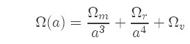
This mini-article deals with the much celebrated Friedmann equation of cosmological expansion. In Part 3 of this mini-series, we had a brief look at the cosmological energy density parameter as a function of the expansion factor (a):

This naturally leads on to the Friedmann equation for the expansion rate of the universe over time:

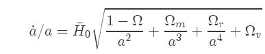
Formidable as it looks, it is actually quite simple to understand, if taken step by step:

is the rate of change of the expansion factor per unit expansion factor. Recall that the expansion factor a is the ratio between how much expansion has happened at any time and the amount of expansion today. The present value of a = 1 and at the Big Bang it was zero.

is somewhat like expressing your car's speed as a fraction of the distance covered. If you drive at a a constant speed, the fraction will shrink as distance covered gets larger. The reason for this unusual ratio will soon become apparent.

(pronounced H-naught-bar) is the Hubble constant, the present expansion rate of the universe. Note that a and all the Ωs are dimensionless, so a-dot and H₀-bar must have the same units, which is inverse time (time^-1). The bar is just to indicate that it is a normalized expansion rate and not the conventional H₀ expressed in conventional units (Km s^-1 Mpc^-1), where Mpc is Mega-parsec.

The square root is a function of the expansion factor and shrinks as a grows larger. Ω is the present total energy density parameter, where Ω = Ω_m+ Ω_r + Ω_v ≈ 1, meaning that the total energy density is very close to the critical density, giving a flat universe.

The other values inside the square root have been discussed in Part 3 and will just be briefly noted: Ω_m, Ω_r, Ω_v are mass energy density, radiation energy density and vacuum energy density respectively.

So what does the Friedmann equation really tell us? (We will reproduce it here, otherwise it tends to scroll off the top...)

The graph below plots the value of the square root as a function of a and the constants: Ω_r = 0.001, Ω_m= 0.2999, Ω_v = 0.7 (so that Ω = 1). For the individual components, it was calculated as if only that component is present, e.g., for matter density, the purple curve, SQRT(Ω_m/a³) was plotted.

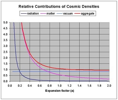
When a << 1, Ω_r/a⁴ (radiation energy density, the dark blue curve) dominated the expansion. A fraction with a very small value to the power 4 below the line can result in a very large value. Due to the scale requirements, it's not very visible on the graph, but just look at the relative slopes and you can easily see that the radiation part will dominate all else for very small a.

As a became larger then about 0.05 (crossover also not visible on the scale of the graph), matter density started to dominate, because Ω_m>> Ω_r. According to our best knowledge, this matter domination phase lasted for more than half the history of the universe.

As a grows larger than about 0.8, and if vacuum energy density is around Ω_v = 0.7, it starts to dominate the value inside the square root. It is easy to see that the other terms under the root get 'diluted' by a > 1. Actually, the square root part will approach the constant value: sqrt(Ω_v) asymptotically as a grows very large.

So much for the right hand side of the Friedmann equation. What does this tell us about the left hand side?

On the left hand side, a, however large, still features below the line. The only way that the left side can also achieve constancy for large a, is for the expansion rate (a-dot) to change in the same sense and magnitude (increasing or decreasing) than what a does.

This explains how the universe could gradually go over from an initially decreasing expansion rate to an increasing expansion rate, provided that there is vacuum energy (a.k.a. dark energy) with positive density.

Does all this tend to bend the mind a bit? Do not feel alone! The cosmology part of the website Relativity 4 Engineers attempts to make it more digestible for engineers. Or you can read Peebles or Peacock (post-grad physical cosmology books)...

Next - how to plot a cosmological expansion curve, using the Friedmann equation...